Car driving performance
table of contents
Car driving performance
When a car runs, multiple resistances occur. The principal among them are rolling resistance, air resistance, grade resistance, and acceleration resistance.
Rolling resistance is caused by the friction between the tires and the road surface, and air resistance is caused by the friction between the tires and the air as the vehicle moves.
Gradient resistance is the resistance caused by gravity when climbing a slope, and acceleration resistance is the force required to increase speed.
All of these resistance forces act in a direction that impedes running, and are collectively called running resistance.
In contrast to running resistance, driving force is the force that allows a vehicle to move forward. This force is generated by the torque generated by the engine, and in order for the car to move forward, this driving force must exceed the running resistance.
Specifically, the power generated by the engine is transmitted to the wheels via the gearbox to move the vehicle. The magnitude and efficiency of this driving force directly affects the vehicle’s acceleration performance and performance on slopes.
- Driving performance curve diagram
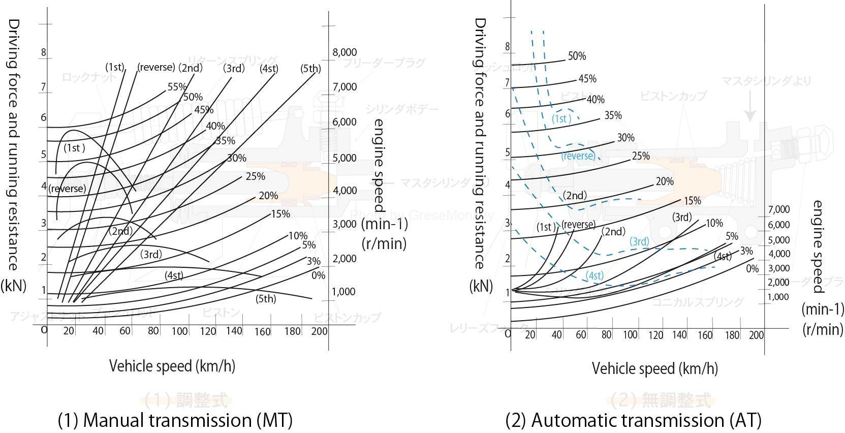
Figure 1: Driving performance curve diagram
The driving performance curve diagram in Figure 1 is a visual representation of the driving performance of a car.
This diagram shows the relationship between vehicle speed, driving force, and engine rotational speed in a diagram. This diagram provides a detailed understanding of the vehicle’s performance, including its acceleration ability, hill-climbing ability, and maximum speed.
For example, it can read how much driving force is generated when the engine rotational speed is constant, or the efficiency of the engine at a specific speed. This provides important information for optimizing vehicle performance.
Running resistance and driving force
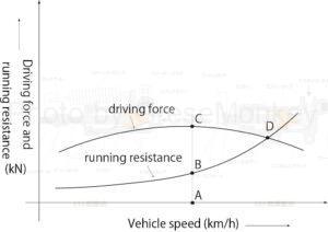
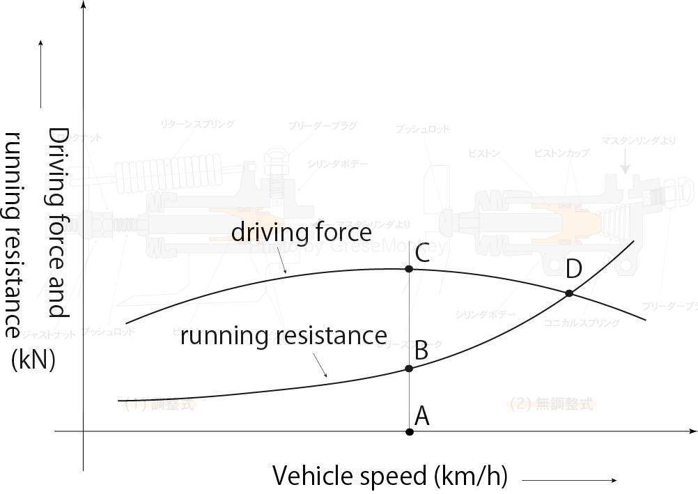
Figure 2: Running resistance and driving force
Figure 2 shows the relationship between the vehicle speed of a car traveling in top gear on a flat road, and the corresponding running resistance and driving force. When the vehicle speed in the diagram is point A, the driving force is located at point C and the running resistance is located at point B. At this time, the driving force C exceeds the running resistance B, and the difference becomes the margin driving force. This surplus driving force acts as an accelerating force when the vehicle travels on a flat road surface.
Marginal driving force = Driving force C - Running resistance B
When the vehicle travels uphill, this extra driving force acts as climbing force. However, as the slope of the slope increases, the slope resistance increases, and as a result, the margin driving force decreases. As the vehicle speed continues to increase, the driving force and running resistance become equal at point D in the diagram, and no further increase in speed occurs and the speed remains constant. The speed at this time is called the maximum speed.
Maximum speed = (driving force = running resistance)
From the above, the relationship between driving force, running resistance, and margin driving force is expressed by the following equation.
Driving force = running resistance + margin driving force
This formula is the basis for numerically understanding vehicle performance, and is an important index when evaluating vehicle acceleration performance and maximum speed.
running resistance
Running resistance is a general term for multiple resistances that a car must overcome when moving. Specifically, it consists of the following four elements.
The resistance that tires receive from the road surface when a car is running
Resistance received from airflow etc. that occurs when a car is running
The resistance that a car experiences when going up or down a hill, etc.
Various resistances experienced when the car accelerates by stepping on the accelerator
These resistances are necessary for vehicles to run efficiently, and directly affect vehicle performance such as energy efficiency, fuel efficiency, acceleration performance, and top speed. When designing a vehicle, it is necessary to minimize these running resistances to maximize performance and reduce fuel consumption.
rolling resistance
Rolling resistance is the resistance force that occurs when a tire rolls on a road surface, and the main cause is energy loss due to contact between the tire and the road surface. It is affected by conditions such as tire material, air pressure, road surface quality, and tire temperature. The rolling resistance increases as the running speed increases, but the rate of increase becomes relatively small.
This resistance is mainly caused by the following factors.
- Deformation of tire contact area
The contact surface of the tire when the car is stationary is called the tire contact area. This area changes depending on the shape and air pressure of the tire, and the area and shape of the contact with the ground also change depending on the quality and shape of the road surface. As the tire rotates, the contact area continuously deforms, and this deformation creates resistance.
- Friction between tires and road surface
When a car is running, the tread portion of the tire comes into contact with the road surface, and frictional force is generated at this contact portion. The amount of friction changes depending on the tire material, tread pattern, road surface condition, etc., and this frictional force causes rolling resistance.
Friction also occurs in the bearing, which is the rotation axis of the tire. This is due to the bearings that connect the wheels and the car body, and the amount of resistance changes depending on the structure and lubrication condition of the bearings themselves. Friction in this area also becomes part of the rolling resistance.
- Impact and deformation from the road surface
Because the road surface is not perfectly flat, when driving over irregular shapes such as bumps and curves, a different resistance occurs than when driving in a normal straight line. This is because tires require additional energy to accommodate the deformation of the road surface.
These factors act comprehensively as tire running resistance, and affect the fuel efficiency and power performance of automobiles. Therefore, it is important to minimize these resistances in vehicle design and maintenance.
Rolling resistance is influenced by the weight of the car and road surface conditions, and there are various factors involved, but rolling resistance on a flat road is generally calculated using the following formula.
$$ R1 = \mu Mg $$
however
\( R1 \):rolling resistance \(N\) = \(kg\)・\(m/s\)\(^2\) = \(kg\)・\(m\)・\(s\)\(^{-2}\)
\( \mu \):rolling resistance coefficient
\( M \):Total vehicle mass(\(kg\))
\( g \):gravitational acceleration = 9.8 \(m/s\)\(^2\) = 9.8\( m\)・\(s\)\(^{-2}\)
Effects of road surface conditions
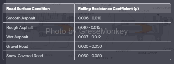
The rolling resistance coefficient is shown in Table 1 below.
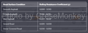
Table 1: Road surface conditions and rolling resistance coefficient
What is the “coefficient” of rolling resistance coefficient?
When a formula with one or more variables is used to explain the regularity of a certain phenomenon, a coefficient is a constant that is applied to the formula using those variables, and the constant changes depending on the situation.
For example, the rolling resistance calculation formula (\(R1 = \mu Mg\)) above has only two variables: the required rolling resistance R1 and the total vehicle mass \(M\).
Among these variables, the rolling resistance \(R1\) can be calculated by multiplying three elements: the coefficient (constant) \(\mu\) which varies depending on the road surface conditions shown in Table 1, the constant gravitational acceleration\(g\)(which is 9.8\(m/s^2\)),and the variable total weight of the automobile \(M\).
Here, when considering determining the rolling resistance of the same car under various road conditions, the total vehicle weight M needs to be a constant value, so it can be treated as a constant instead of a variable.
If you can select the road surface condition and determine the value of μ, which is the rolling resistance coefficient, then all you have to do is substitute each value into the formula \(R1 = \mu Mg\), and the rolling resistance will inevitably be determined. determined.
Effect of vehicle speed
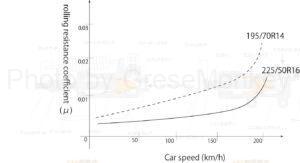
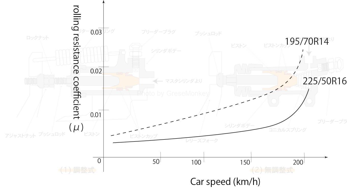
Figure 3: Relationship between vehicle speed and rolling resistance coefficient
As shown in Figure 3, the rolling resistance coefficient tends to increase rapidly when the vehicle speed exceeds a certain level.
This is due to the generation of standing waves in the tires.
Standing wave is a phenomenon that occurs when a tire is continuously subjected to a load. Automobile tires always maintain a deflected state due to the load of the vehicle.
Tire deflection will be greater if the tire pressure is incorrect or if the vehicle is overloaded and heavy. If the vehicle continues to drive at high speeds in this state, multiple deflections will overlap inside the tire, creating a standing wave. If this condition continues, it may cause serious trouble such as tire burst.
However, even if the tire pressure is appropriate, standing waves can occur when driving at high speeds.
This is because tires are not perfectly round, and even when they are in proper condition, they are slightly bent. Even if the driver is not aware of it, this deflection can cause standing waves.
However, tires are designed and developed in such a way that they do not cause any trouble even when driving at a certain high speed, assuming appropriate air pressure and mounting conditions. Therefore, it is important to properly maintain and regularly check your tires, which can prevent problems caused by standing waves.
Effect of tire deformation amount
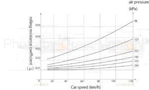
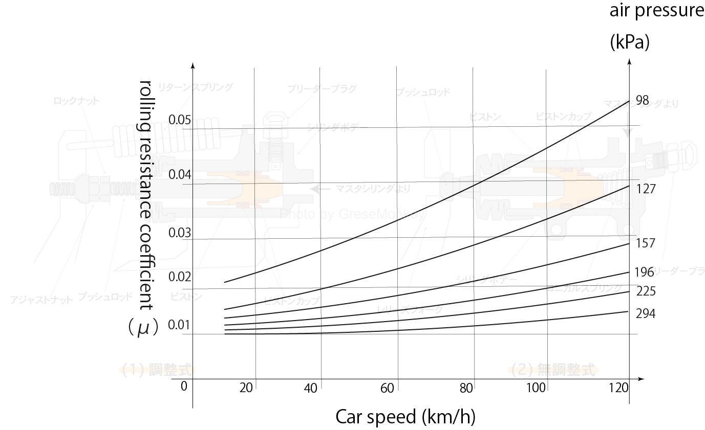
Figure 4: Relationship between tire air pressure, vehicle speed, and rolling resistance coefficient
The higher the tire air pressure, the smaller the tire deformation, and therefore the smaller the rolling resistance coefficient.
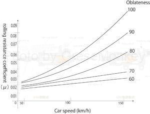
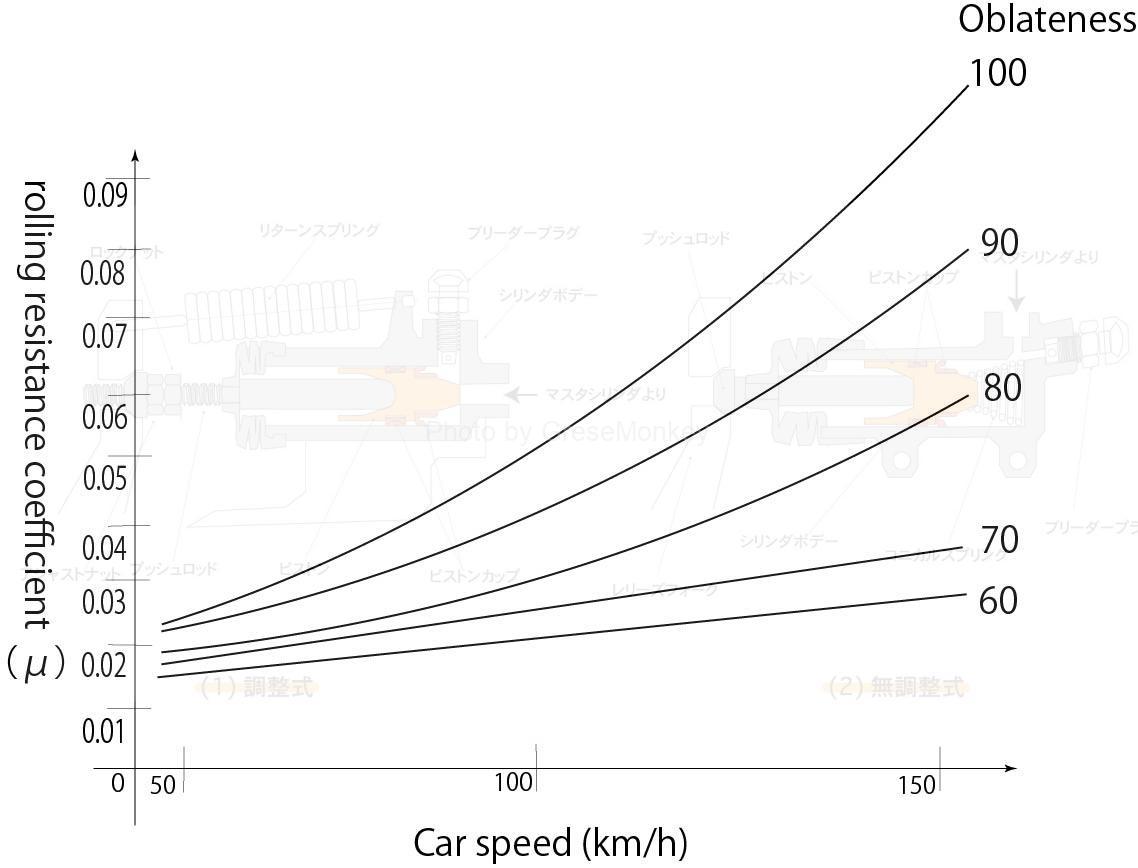
Figure 5: Relationship between aspect ratio and rolling resistance coefficient
The smaller the tire’s aspect ratio, the smaller the tire deformation, and therefore the smaller the rolling resistance coefficient.
Tire aspect ratio

        Tire aspect ratio(%) = (Tire section height / Section width) * 100
Simply put, the tire’s flatness is the flatness of the tire. In other words, when the tire is viewed from the side, the lower the height between the wheel end face and the tire end face, the lower the tire’s aspect ratio. Most tires have a wide tread (tread) and are made harder than normal tires, so there is little deformation of the tires even when driving at high speeds, and they also have good running stability.
On the other hand, tires with high profile ratios have a long distance from the wheel edge to the tire edge, and are made softer to absorb shock. As a result, they tend to deform and increase rolling resistance when driving at high speeds, but they provide better ride comfort than tires with a lower profile ratio.
Impact of slope
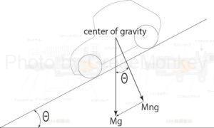
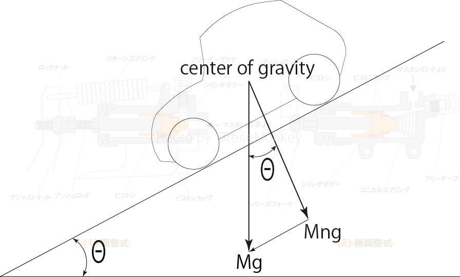
Figure 6: Vertical load on slope
On a slope as shown in Figure 6, the load perpendicular to the slope road surface (\(Mng\)), which is a component of the total vehicle mass * gravitational acceleration (\(Mg\)), decreases as the slope angle \(\theta\) increases.
This relationship is expressed by the following equation.
$$Mng = Mg\cos\theta$$
Therefore, the rolling resistance of the slope \(R1\) ,
$$R1 = \mu Mg \cos\theta$$
however
\(R1\):Rolling resistance on slopes \(N\)=\(kg\)\(m/s\)\(^2\)
\(\mu\):rolling resistance coefficient
\(M\):Total vehicle mass
\(g\):gravitational acceleration \(9.8m/s\)\(^2\)
\(\theta\):slope angle
air resistance
Air resistance is the resistance that occurs when a car displaces air and changes depending on factors such as the shape of the car, the smoothness of its surface, and the speed of the car. As speed increases, the force of air resistance increases in proportion to the square of speed, so the faster you drive, the greater the effect.
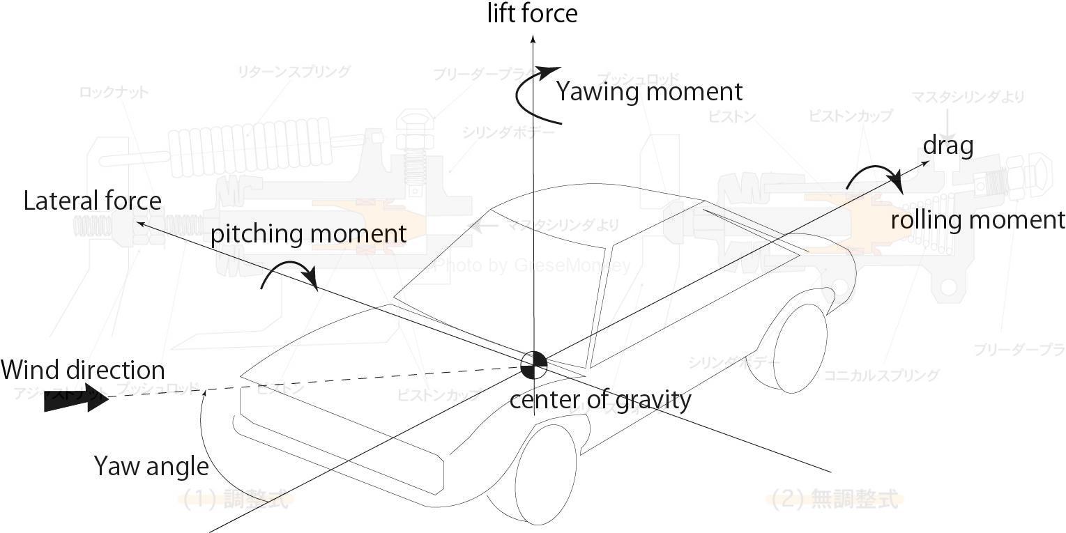
When the vehicle is traveling straight and there is no natural wind, drag (force opposite to the direction of travel), lift (force trying to rise), and lateral force (force perpendicular to the direction of travel) act on the vehicle body.
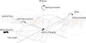
Figure 7: Forces acting on the car body
As shown in Figure 7, when natural wind blows or the car turns, in addition to the forces in the three directions (drag, lift, and lateral force) shown in this diagram, yawing moment, rolling moment, and pitching moment are generated. As a result, the maneuverability and stability of the vehicle will be greatly affected.
Drag, lift, and lateral forces are the three main aerodynamic forces that affect vehicle motion.
Drag force is a force that acts rearward on the vehicle body. As the car moves forward, the air received at the front of the car body creates positive pressure, while the separation of air at the rear creates negative pressure. The combination of these positive and negative pressures acts as a force that pulls the vehicle backwards, that is, a drag force. This drag increases in proportion to vehicle speed, and has a direct impact on fuel efficiency and top speed.
Lift is a force that acts perpendicularly upward on the vehicle body. The difference in pressure created by the difference in speed of air flowing between the top and bottom of the car body creates a force that lifts the car body. As the lift force increases, the ground contact force of the tire with the road surface decreases, thereby reducing steering stability. Lift is often a problem, especially when driving at high speeds, and in racing cars and high-performance cars, aerodynamic design is emphasized in order to suppress this lift.
Lateral force is a force that acts in the lateral direction of the vehicle body. This force is mainly caused by crosswinds and increases in proportion to changes in wind direction (yaw angle). Lateral forces can cause the vehicle to skid or change its direction of travel, leading to unexpected behavior for the driver. The effect of crosswinds is particularly large on expressways, and disturbances in steering due to lateral forces have a direct impact on driving safety.
Air resistance is proportional to the front projected area of the vehicle and the square of the airspeed, and is expressed by the following formula.
$$R2 = \frac{1}{2} Cd Av^2\rho$$
however
\(R2\):air resistance \(N\) = \(kg\)・\(m/s\)\(^2\)
\(Cd\):air resistance coefficient
\(A\):Full projected area \(m\)\(^2\)
\(v\):airspeed \(m/s\)
\(\rho\):air density \(kg/m\)\(^3\)
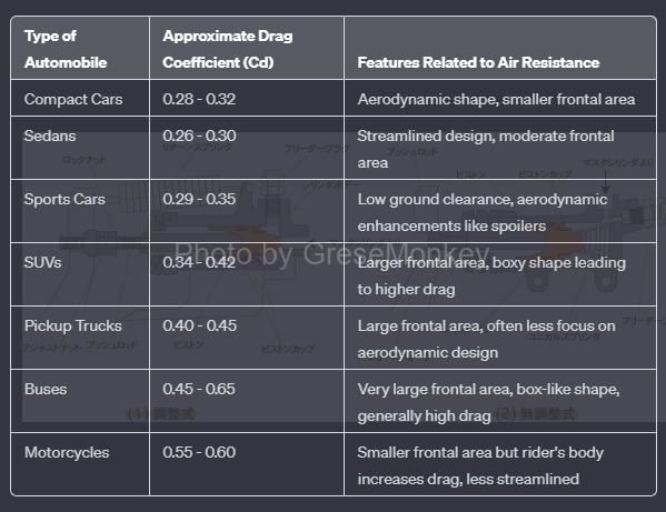
Note that the air resistance coefficient varies depending on the shape of the vehicle body (Table 2)
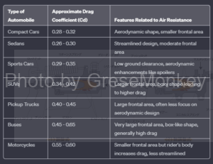
Table 2: Air resistance coefficient of automobiles
Note 1) Airspeed: The composite speed of the vehicle speed and wind speed.
Note 2) Air density is standard standby condition(1 atm/15℃), 1.225kg/m\(^2\)
gradient resistance
Gradient resistance is the resistance that occurs when climbing a slope, and is related to the magnitude of the slope and gravity. This resistance is directly proportional to the slope angle and independent of vehicle speed. The steeper the slope, the greater the grade resistance.
When a car goes up a hill, the force of the car’s weight acts in the opposite direction to the driving force.
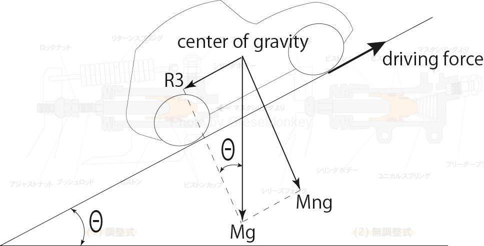
This is called gradient resistance. As shown in Figure 8, when a car with a weight (\(Mg\)) climbs a slope with a slope angle \(\theta\), the component force of gravity (\(R3\)) is the slope resistance and is expressed by the following formula.
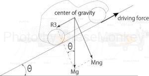
Figure 8: Gradient and slope resistance
$$R3 = Mg・sin\theta$$
however
\(R3\):gradient resistance \(N\) = \(kg\)・\(m/s\)\(^2\)
\(M\):Total vehicle mass \(kg\)
\(g\):gravitational acceleration = 9.8\(m/s\)\(^2\)
\(\theta\):slope angle
The slope of a road is generally expressed as \(\tan\theta\), so to calculate slope resistance, it is necessary to find \(sin\theta\) from \(tan\theta\).
However, when \(\theta\) is small, there is no practical problem in approximately assuming that \(sin\theta ≒ tan\theta\).
For example, when calculating the slope resistance when a car with a total mass of 1225 kg goes up a 10% slope.
Considering \(\tan\theta ≒ \sin\theta\),
Since \(\tan\theta = 0.1\), \(\sin\theta = 0.1\)
From the gradient resistance \(R3 = Mg \cdot \sin\theta\)
\(R3 = 1225 \, \text{kg} \times 9.8 \, \text{m/s}^2 \times 0.1 = 1200.5 \, \text{N}\)
Therefore \(R3 = 1200.5 \, \text{N}\)
From the above, it follows that the car is being subjected to the same gradient resistance that is being pulled backwards by a force of approximately 1200N.
This is because the work of lifting the mass of the vehicle to a high position is added as the vehicle travels.
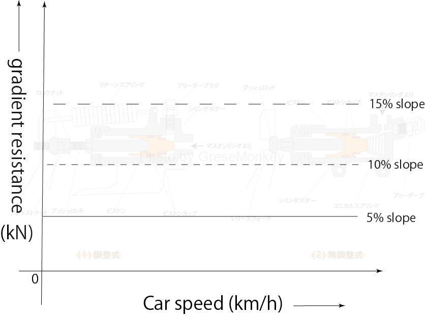
The slope resistance is a constant value regardless of the vehicle speed, but as the slope changes, the resistance also changes, resulting in the characteristics shown in FIG. 9.
Note that in the case of a downhill slope, the slope resistance becomes negative and reduces the running resistance, so it acts as a force to assist the driving force.
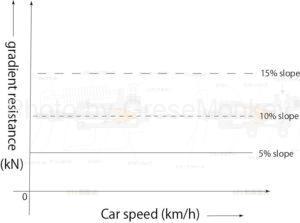
Figure 9: Gradient resistance on an uphill slope
acceleration resistance
The resistance that occurs when a car accelerates is called acceleration resistance, which is the resistance that occurs against the force that attempts to accelerate due to the law of inertia.
Acceleration resistance is the additional force required when a car accelerates, and force is needed to overcome inertia in order for a car to change speed. The magnitude of this resistance is determined by the degree to which the accelerator is depressed and the acceleration of the vehicle, and is also influenced by the driver’s driving technique. The more rapid the acceleration, the greater the acceleration resistance.
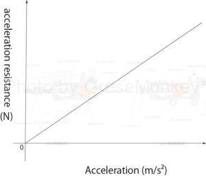
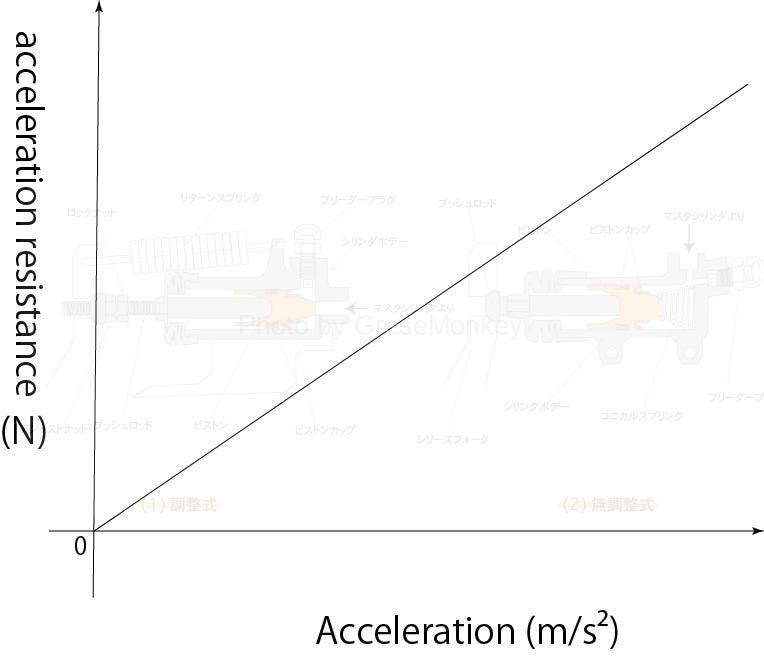
Figure 10: Relationship between acceleration resistance and acceleration
Therefore, this acceleration resistance acts in the direction of decelerating the accelerated automobile.
Acceleration resistance is expressed by the following formula.
$$R4 = M\alpha + M’\alpha = (M + M’)\alpha$$
however
\(R4\):acceleration resistance \(\text{N} = \text{kg} \cdot \text{m/s}^2 = \text{kg} \cdot \text{m} \cdot \text{s}^{-2}\)
\(\alpha\):acceleration \(\text{m/s}^2\)
\(M\):Total vehicle mass \(\text{kg}\)
\(M’\):Inertial mass equivalent to rotating part \(\text{kg}\)
Driving power and driving performance
If the driving force can be increased, the ability to climb hills and accelerate will increase, and the maximum speed will also increase.
The driving force can be increased by increasing the engine torque or the reduction ratio of the power transmission, or by decreasing the diameter of the drive wheels.
However, if the driving force exceeds the frictional force between the road surface and the tires, the vehicle will spin, and power cannot be transmitted effectively.
Therefore, the maximum limit of driving force can be expressed by the following formula.
$$F0 = \mu Mg$$
however
\(F0\):Maximum limit of driving force \(\text{N} = \text{kg} \cdot \text{m/s}^2 = \text{kg} \cdot \text{m} \cdot \text{s}^{-2}\)
\(\mu\):Coefficient of friction between the road surface and tires
\(M\):Total mass on drive wheels \(\text{kg}\)
\(g\):gravitational acceleration \(9.8 \, \text{m/s}^2 = 9.8 \, \text{m} \cdot \text{s}^{-2}\)
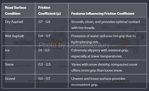
The coefficient of friction (\(\mu\)) changes depending on the road surface and tire conditions. (Table 3)
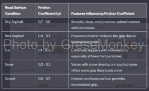
Table 3: Friction coefficient
There is a limit to the driving force for each drive wheel.
Four-wheel drive (4WD) systems are advantageous in maximizing driving performance such as hill-climbing ability, acceleration ability, and maximum speed, but there are also ways to reduce running resistance by improving the shape and materials of the vehicle. It will be effective to minimize it.
Driving performance
Driving performance curve diagram
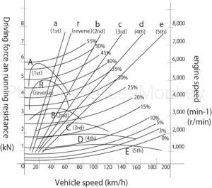
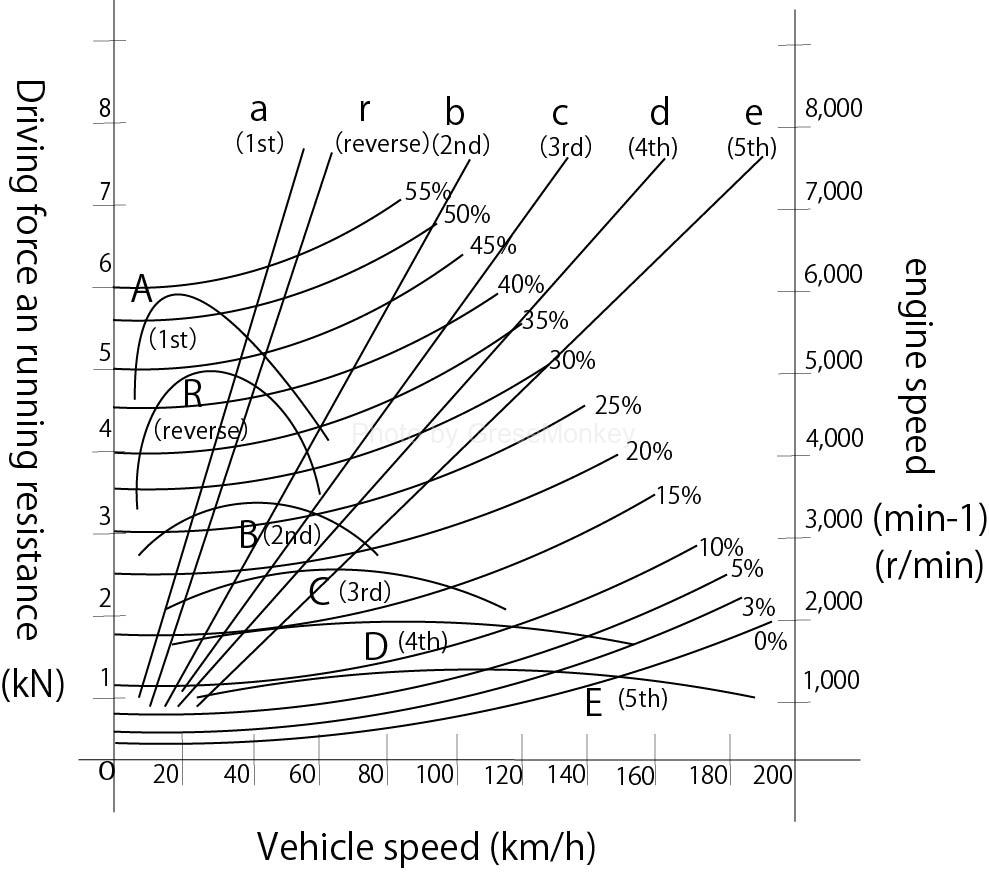
Figure 11: Driving performance curve diagram
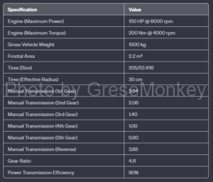
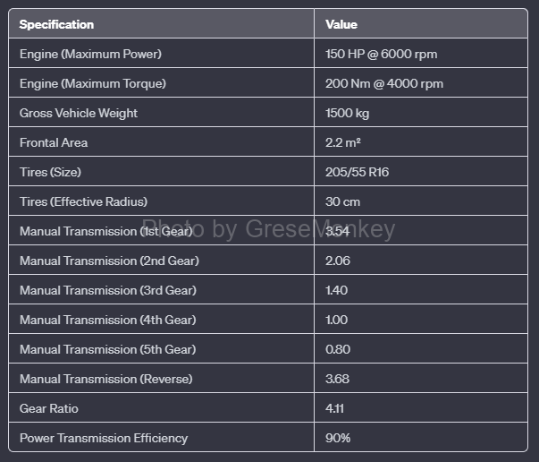
Table 4: General car specifications table
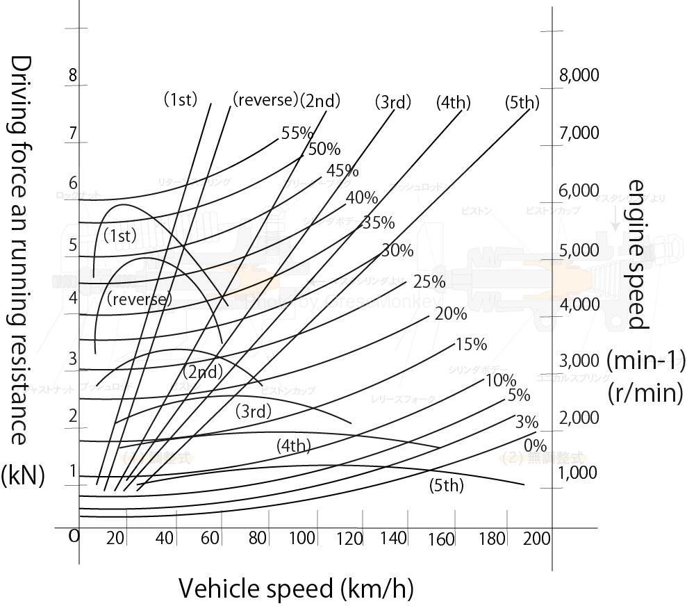
FIG. 11 shows a driving performance curve diagram of an automobile having the performance shown in the specification table of Table 4.
The horizontal axis is the vehicle speed (\(km/h\)), and the vertical axis is the driving force and running resistance (\(kN\)) and engine rotation speed (\(\text{min}^{-1}\)). It shows.
The elements shown in FIG. 11 are as follows.
-
- A~E and R are the driving forces at vehicle speeds from 1st to 5th shift and reverse, respectively.
- 0~55% is running resistance at vehicle speed on uphill slopes
- a~e and r are engine rotational speeds at vehicle speed
- Relationship with engine performance curve
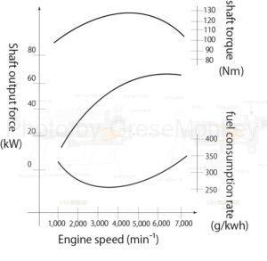
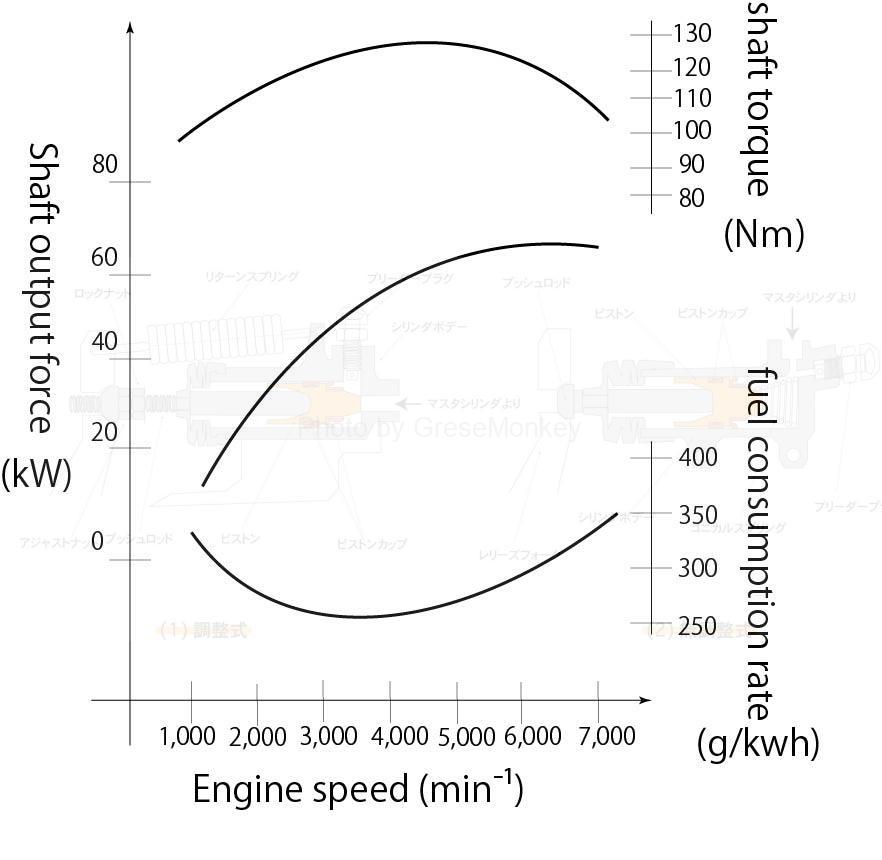
Figure 12: Engine performance curve diagram
FIG. 12 is an engine performance curve diagram of the automobile shown in the driving performance curve diagram of FIG. 11.
From Figure 12, it can be seen that this engine, with a rotational speed of 1000~6500\(\text{min}^{-1}\), outputs a shaft torque of approximately 90 to 120\(N・m\) in this range.
Generally, the following relationship exists between engine torque and vehicle driving force.
$$F = \frac{Te \cdot i \cdot \eta}{r}$$
however
\(F\):driving force \(\text{N}\)
\(Te\):engine torque \(\text{N} \cdot \text{m}\)
\(i\):Total reduction ratio
\(\eta\):Power transmission efficiency
\(r\):Dynamic load radius of drive wheel tires \(\text{m}\)
From this equation, it can be seen that the driving force of an automobile is proportional to the engine torque, total reduction ratio, and power transmission efficiency, and inversely proportional to the dynamic load radius of the drive wheel tires.
Further, there is the following relationship between the engine rotation speed and the vehicle speed.
The distance the car travels during one revolution of the drive wheels is \(2\pi r\) [\(m\)], where \(r\) [\(m\)] is the tire’s dynamic load radius.
In other words, if the drive wheel rotates \(Nr\) [\(\text{min}^{-1}\)], the distance traveled in one hour will be \(Nr \cdot 60\) [\(\text{h}^{-1}\)] \(\cdot 2\pi r\) [\(m\)].
Therefore, to find vehicle speed (\(v\)) by \(km/h\) (conversion), divide by \(10^3\) [\(m\)] \(\cdot\) [\(\text{km}^{-1}\)].
\(v = \frac{Nr \cdot 60 \cdot 2\pi r}{10^3}\) [\(km/h\)]
Therefore \(v = \frac{Nr \cdot 60 \cdot 2\pi r}{10^3}\) [\(km/h\)] —➀
Also, \(Nr = \frac{Ne}{i}\) (engine speed) , the relationship between engine rotation speed and vehicle speed is
Substituting \(Nr = \frac{Ne}{i}\) for \(v = \frac{Nr \cdot 60 \cdot 2\pi r}{10^3}\) [\(km/h\)], we get
\(v = \frac{Ne \cdot 60 \cdot 2\pi r}{10^3 \cdot i}\) [\(km/h\)]
Therefore \(v = \frac{Ne \cdot 60 \cdot 2\pi r}{10^3 \cdot i}\) [\(km/h\)] —➁
By applying the specification table in Table 4 and the engine rotation speed and torque values in FIG. 12 to these two equations ➀ and ➁, it is possible to calculate the relationship between vehicle speed, driving force, and engine rotation speed.
Furthermore, when looking at the relationship between driving force, vehicle speed, and output, the following equation holds true.
$$P = Fv$$
however
\(P\):output \(\text{W} = \text{kg} \cdot \text{m}^2/\text{s}^3 = \text{kg} \cdot \text{m}^{-2} \cdot \text{s}^{-3}\)
\(F\):driving force \(\text{N} = \text{kg} \cdot \text{m/s}^2 = \text{kg} \cdot \text{m} \cdot \text{s}^{-2}\)
\(v\):Vehicle speed \(\text{m/s} = \text{m} \cdot \text{s}^{-1}\)(For km/h display, use \(\frac{1}{3.6} \cdot v\) [\(\text{m} \cdot \text{s}^{-1}\)])
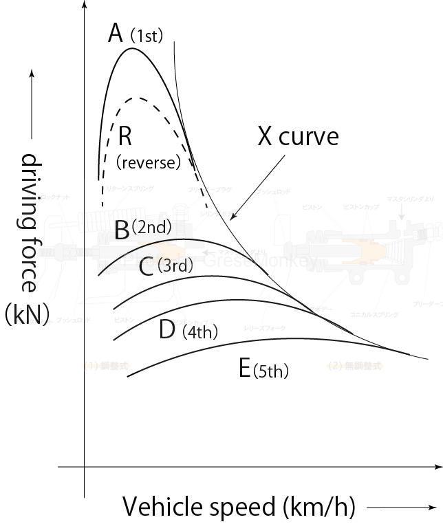
The driving force curve, as shown in A (1st speed) in Fig. 13, has a large driving force in 1st speed, but the speed range is narrow and is biased to the left.
Also, the driving force curve gradually becomes lower and wider from A to E.
Note that in the case of a continuously variable transmission such as a CVT, the transmission will be as shown in the X curve in the figure.
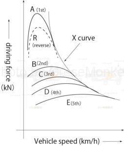
Figure 13: Relationship of driving force between 5-speed forward transmission type and continuously variable transmission type
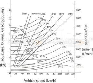
Figure 11: Driving performance curve diagram
In the driving performance curve diagram of FIG. 11, each line from 0 to 55% is a curve showing uphill driving performance, and % represents the magnitude of the slope.
For example, 20% indicates the slope of \(tan\)\(\theta\)=0.2(\(\theta\) is slope angle), and the 0% line is a curve that indicates running resistance on a flat road surface, which is the sum of rolling resistance and air resistance.
maximum speed
Figure 11: Driving performance curve diagram
The maximum speed of an automobile generally refers to the intersection of the driving force curve and the running resistance curve when driving on a flat road surface in the gear with the smallest transmission ratio.
Therefore, it can be seen from the intersection of the 5th speed driving force curve and the 0% running resistance curve that the maximum speed of a car with the performance shown in the running performance curve diagram of FIG. 11 is approximately 165 km/h.
acceleration performance
Figure 11: Driving performance curve diagram
In FIG. 11, considering the case of running on a flat road, the driving force is greater than the running resistance below the maximum speed, so the difference is used for acceleration as extra driving force.
The extra driving force is greatest in 1st gear and decreases in the order of 2nd, 3rd, 4th, and 5th gears, so if you shift appropriately from 1st to 5th gear, you can obtain a large acceleration.
The acceleration when the vehicle is traveling at a given speed can be calculated from the traveling performance curve diagram.
The relationship between acceleration (\(\alpha\)) and acceleration force (\(F\)) is
\(F = (M + M’)\alpha \, [\text{N}]\) or \(\alpha = \frac{F}{M + M’} \, [\text{m/s}^2]\)
For example, in Figure 11, when driving at 70 km/h on a flat road in 3rd gear, the extra driving force is approximately 1.7 kN. From Table 4, the total mass of the car is 1225 kg, so the acceleration can be calculated as follows.
car mass = \(1225 \, [\text{kg}] – 55 \, [\text{kg/person}] \times 5 \, [\text{person}] = 950 \, [\text{kg}]\) (Total vehicle mass – Vehicle mass)
If \(M’\) is 5% of the vehicle mass, then
\(M’ = 950 \, [\text{kg}] \times 0.05 = 47.5 \, [\text{kg}]\)
from \( \alpha = \frac{F}{M + M’} \, [\text{m/s}^2] \)
acceleration \( \alpha = \frac{1.7 \times 10^3 \, [\text{kg} \cdot \text{m} \cdot \text{s}^{-2}]}{1225 \, [\text{kg}] + 47.5 \, [\text{kg}]} = \frac{1700 \, [\text{kg} \cdot \text{m} \cdot \text{s}^{-2}]}{1272.5 \, [\text{kg}]} \approx 1.34 \, [\text{m/s}^2]\)
\( \alpha = 1.34 \, [\text{m/s}^2] \)
Therefore, it can be seen that in order to improve acceleration performance, it is necessary to increase the margin driving force (increase acceleration) and reduce the total mass of the vehicle (reduce weight).
Climbing ability
When going up a slope at a constant speed
Driving force – (rolling resistance + air resistance) = \(F\)
This force (\(F\)) is all spent on gradient resistance, so
\(F = Mg\sin\theta\)
From this formula, the slope angle \(\theta\) of the slope that can be climbed can be determined.
Furthermore, in the running performance curve diagram, the speed at which the vehicle can climb the gradient at each shift stage can be determined from the intersection of the running resistance curve for each gradient and the driving force curve at each shift stage.